Background
Motivation
I am currently reading the book “Machine Learning with R”1 by Brent Lantz,
and also want to learn more about the caret2 package, so I decided to replicate
the kNN example from the chapter 3 of the book using caret instead of the
class3 package used in the text.
Preliminary information
The dataset used in the book is a modified version of the “Breast Cancer Wisconsin (Diagnostic) Data Set” from the UCI Machine Learning Repository4, as described in Chapter 3 (”*Lazy Learning – Clasification Using Nearest Neighbors”) of the aforementioned book.
You can get the modified dataset from the book’s page at Packt, but be aware that you will need to register to get the files. If you rather don’t do that, you can get the original data files from the UCI repository, in particular you need to get the files:
- https://archive.ics.uci.edu/ml/machine-learning-databases/breast-cancer-wisconsin/wdbc.data
- Contains the 569 diagnosis
- https://archive.ics.uci.edu/ml/machine-learning-databases/breast-cancer-wisconsin/wdbc.names
- Contains a complete description of the dataset, including relevant references
If you are going to use the original dataset, be aware that it doesn’t have a header row, also, you might want to randomize it a bit. Something like the following code might work (feel free to improve it):
uciurl <- "https://archive.ics.uci.edu/ml/machine-learning-databases/breast-cancer-wisconsin/wdbc.data"
download.file(url=uciurl, destfile="wdbc.data", method="curl")
wdbc <- read.csv("wdbc.data", header=FALSE, stringsAsFactors=FALSE)[-1]
wdbc <- wdbc[sample(nrow(wdbc)),]
features <- c("radius", "texture", "perimeter", "area", "smoothness",
              "compactness", "concavity", "concave_points", "symmetry",
              "fractal_dimension")
calcs <- c("mean", "se", "worst")
colnames(wdbc) <- c("diagnosis",
                    paste0(rep(features, 3), "_", rep(calcs, each=10)))
For this excercise we will use the caret package to do the kNN modeling and
prediction, the pander package to be able to output nicely formated tables,
and the doMC to take advantage of parallel processing with multiple cores.
Also, we will define some utility functions to simplify matters later in the code.
library(caret)
library(pander)
library(doMC)
registerDoMC(cores=4)

# a utility function for % freq tables
frqtab <- function(x, caption) {
    round(100*prop.table(table(x)), 1)
}

# utility function to round values in a list
# but only if they are numeric
round_numeric <- function(lst, decimals=2) {
    lapply(lst, function(x) {
        if (is.numeric(x)) {
            x <- round(x, decimals)
        }
        x
        })
}

# utility function to summarize model comparison results
summod <- function(cm, fit) {
    summ <- list(k=fit$finalModel$k,
                 metric=fit$metric,
                 value=fit$results[fit$results$k == fit$finalModel$k, fit$metric],
                 TN=cm$table[1,1],  # true negatives
                 TP=cm$table[2,2],  # true positives
                 FN=cm$table[1,2],  # false negatives
                 FP=cm$table[2,1],  # false positives
                 acc=cm$overall["Accuracy"],  # accuracy
                 sens=cm$byClass["Sensitivity"],  # sensitivity
                 spec=cm$byClass["Specificity"],  # specificity
                 PPV=cm$byClass["Pos Pred Value"], # positive predictive value
                 NPV=cm$byClass["Neg Pred Value"]) # negative predictive value
    round_numeric(summ)
}
Reading and preparing the data
As the first column in the original CSV file contains only an id, which we will not use, we read the csv and remove it before assigning it to a data frame.
Also, we will convert the diagnosis to a factor, in a similar fashion as the example in the book.
# You may want to omit the next line if using the UCI dataset
wdbc <- read.csv("wisc_bc_data.csv", stringsAsFactors = FALSE)[-1]
# recode diagnosis as a factor -- as done in the book example
wdbc$diagnosis <- factor(wdbc$diagnosis, levels = c("B", "M"),
                         labels = c("Benign", "Malignant"))
str(wdbc)
'data.frame':    569 obs. of  31 variables:
 $ diagnosis        : Factor w/ 2 levels "Benign","Malignant": 1 1 1 1 1 1 1 2 1 1 ...
 $ radius_mean      : num  12.3 10.6 11 11.3 15.2 ...
 $ texture_mean     : num  12.4 18.9 16.8 13.4 13.2 ...
 $ perimeter_mean   : num  78.8 69.3 70.9 73 97.7 ...
 $ area_mean        : num  464 346 373 385 712 ...
 $ smoothness_mean  : num  0.1028 0.0969 0.1077 0.1164 0.0796 ...
 $ compactness_mean : num  0.0698 0.1147 0.078 0.1136 0.0693 ...
 $ concavity_mean   : num  0.0399 0.0639 0.0305 0.0464 0.0339 ...
 $ points_mean      : num  0.037 0.0264 0.0248 0.048 0.0266 ...
 $ symmetry_mean    : num  0.196 0.192 0.171 0.177 0.172 ...
 $ dimension_mean   : num  0.0595 0.0649 0.0634 0.0607 0.0554 ...
 $ radius_se        : num  0.236 0.451 0.197 0.338 0.178 ...
 $ texture_se       : num  0.666 1.197 1.387 1.343 0.412 ...
 $ perimeter_se     : num  1.67 3.43 1.34 1.85 1.34 ...
 $ area_se          : num  17.4 27.1 13.5 26.3 17.7 ...
 $ smoothness_se    : num  0.00805 0.00747 0.00516 0.01127 0.00501 ...
 $ compactness_se   : num  0.0118 0.03581 0.00936 0.03498 0.01485 ...
 $ concavity_se     : num  0.0168 0.0335 0.0106 0.0219 0.0155 ...
 $ points_se        : num  0.01241 0.01365 0.00748 0.01965 0.00915 ...
 $ symmetry_se      : num  0.0192 0.035 0.0172 0.0158 0.0165 ...
 $ dimension_se     : num  0.00225 0.00332 0.0022 0.00344 0.00177 ...
 $ radius_worst     : num  13.5 11.9 12.4 11.9 16.2 ...
 $ texture_worst    : num  15.6 22.9 26.4 15.8 15.7 ...
 $ perimeter_worst  : num  87 78.3 79.9 76.5 104.5 ...
 $ area_worst       : num  549 425 471 434 819 ...
 $ smoothness_worst : num  0.139 0.121 0.137 0.137 0.113 ...
 $ compactness_worst: num  0.127 0.252 0.148 0.182 0.174 ...
 $ concavity_worst  : num  0.1242 0.1916 0.1067 0.0867 0.1362 ...
 $ points_worst     : num  0.0939 0.0793 0.0743 0.0861 0.0818 ...
 $ symmetry_worst   : num  0.283 0.294 0.3 0.21 0.249 ...
 $ dimension_worst  : num  0.0677 0.0759 0.0788 0.0678 0.0677 ...
Just to have a base measure, let’s look at the the frequencies for the diagnosis
ft_orig <- frqtab(wdbc$diagnosis)
pander(ft_orig, style="rmarkdown", caption="Original diagnosis frequencies (%)")
Original diagnosis frequencies (%)
| Benign | Malignant |
|---|---|
| 62.7 | 37.3 |
Modelling using the book’s data partition and kNN
Using accuracy as metric
In the book, the first 469 rows are assigned to the training set, and the rest to the test set (Note: I am using the book’s modified dataset, if using the the UCI original data, your results might be different)
wdbc_train <- wdbc[1:469,]
wdbc_test <- wdbc[470:569,]
Just for completeness, let’s check if that data partition strategy gives us sets with similar distributions as the original data.
ft_train <- frqtab(wdbc_train$diagnosis)
ft_test <- frqtab(wdbc_test$diagnosis)
ftcmp_df <- as.data.frame(cbind(ft_orig, ft_train, ft_test))
colnames(ftcmp_df) <- c("Original", "Training set", "Test set")
pander(ftcmp_df, style="rmarkdown",
             caption="Comparison of diagnosis frequencies (in %)")
Comparison of diagnosis frequencies (in %)
| Original | Training set | Test set | |
|---|---|---|---|
| Benign | 62.7 | 63.1 | 61 |
| Malignant | 37.3 | 36.9 | 39 |
The frequencies of diagnosis in the tranining set looks a lot like the original data, but the test set contains an bit more malignant diagnosis propotionally.
In spite of this disparity, let’s try to use kNN5 on the sets. We will
use repeated cross-validation, and scale the data using the range
method.
The example in the book does the modelling at several discrete values of k,
here caret provides the means to do that optimization automatically using
a selection metric to decide which model is optimal. We will use Accuracy as
the metric.
ctrl <- trainControl(method="repeatedcv", number=10, repeats=3)
set.seed(12345)
knnFit1 <- train(diagnosis ~ ., data=wdbc_train, method="knn",
                trControl=ctrl, metric="Accuracy", tuneLength=20,
                preProc=c("range"))
knnFit1
k-Nearest Neighbors

469 samples
 30 predictors
  2 classes: 'Benign', 'Malignant'

Pre-processing: re-scaling to [0, 1]
Resampling: Cross-Validated (10 fold, repeated 3 times)

Summary of sample sizes: 422, 423, 422, 423, 422, 422, ...

Resampling results across tuning parameters:

  k   Accuracy  Kappa   Accuracy SD  Kappa SD
   5  0.9644    0.9231  0.02524      0.05431
   7  0.9687    0.9321  0.01996      0.04358
   9  0.9715    0.9382  0.01797      0.03903
  11  0.9708    0.9364  0.01903      0.04162
  13  0.9716    0.9379  0.01885      0.04143
  15  0.9659    0.9251  0.02288      0.05130
  17  0.9652    0.9235  0.02349      0.05264
  19  0.9623    0.9172  0.02558      0.05701
  21  0.9580    0.9080  0.02546      0.05616
  23  0.9552    0.9016  0.02536      0.05673
  25  0.9530    0.8968  0.02542      0.05702
  27  0.9523    0.8952  0.02614      0.05874
  29  0.9509    0.8921  0.02456      0.05533
  31  0.9516    0.8936  0.02312      0.05213
  33  0.9531    0.8967  0.02409      0.05422
  35  0.9524    0.8952  0.02553      0.05738
  37  0.9524    0.8953  0.02484      0.05565
  39  0.9524    0.8953  0.02484      0.05565
  41  0.9509    0.8920  0.02580      0.05802
  43  0.9516    0.8935  0.02443      0.05499

Accuracy was used to select the optimal model using  the largest value.
The final value used for the model was k = 13.
plot(knnFit1)
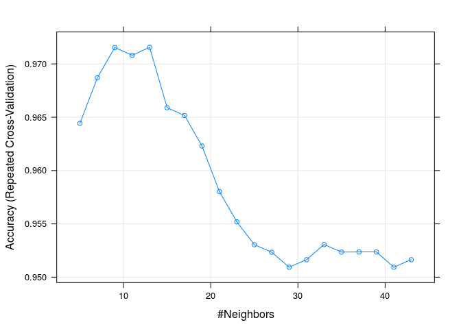
As we can see from the results and plot, by using the accuracy metric and the book’s data partition, the best model is the one with k=13.
Let’s use this model to predict the diagnosis in the test set, and then calculate the corresponding confusion matrix:
knnPredict1 <- predict(knnFit1, newdata=wdbc_test)
cmat1 <- confusionMatrix(knnPredict1, wdbc_test$diagnosis, positive="Malignant")
cmat1
Confusion Matrix and Statistics

           Reference
Prediction  Benign Malignant
  Benign        61         3
  Malignant      0        36

               Accuracy : 0.97
                 95% CI : (0.915, 0.994)
    No Information Rate : 0.61
    P-Value [Acc > NIR] : <2e-16

                  Kappa : 0.936
 Mcnemar's Test P-Value : 0.248

            Sensitivity : 0.923
            Specificity : 1.000
         Pos Pred Value : 1.000
         Neg Pred Value : 0.953
             Prevalence : 0.390
         Detection Rate : 0.360
   Detection Prevalence : 0.360
      Balanced Accuracy : 0.962

       'Positive' Class : Malignant
Using kappa as metric
Let’s find out if the model changes if we use the same data partition, but this
time we use kappa as the model selection metric.
knnFit2 <- train(diagnosis ~ ., data=wdbc_train, method="knn",
                trControl=ctrl, metric="Kappa", tuneLength=20,
                preProc=c("range"))
knnFit2
k-Nearest Neighbors
469 samples
30 predictors
2 classes: 'Benign', 'Malignant'
Pre-processing: re-scaling to [0, 1]
Resampling: Cross-Validated (10 fold, repeated 3 times)
Summary of sample sizes: 422, 422, 423, 422, 422, 421, ...
Resampling results across tuning parameters:
k Accuracy Kappa Accuracy SD Kappa SD
5 0.9644 0.9226 0.02533 0.05575
7 0.9666 0.9273 0.02426 0.05333
9 0.9701 0.9349 0.02223 0.04900
11 0.9695 0.9333 0.02604 0.05725
13 0.9673 0.9282 0.02557 0.05669
15 0.9651 0.9233 0.02827 0.06270
17 0.9645 0.9216 0.02867 0.06390
19 0.9580 0.9074 0.02994 0.06673
21 0.9559 0.9028 0.03175 0.07067
23 0.9545 0.8998 0.03210 0.07136
25 0.9531 0.8967 0.03144 0.06993
27 0.9531 0.8966 0.03144 0.06990
29 0.9531 0.8966 0.03144 0.06990
31 0.9530 0.8966 0.03243 0.07184
33 0.9530 0.8965 0.03243 0.07210
35 0.9545 0.8996 0.03162 0.07031
37 0.9538 0.8980 0.03174 0.07064
39 0.9538 0.8980 0.03174 0.07064
41 0.9538 0.8980 0.03174 0.07064
43 0.9530 0.8964 0.03102 0.06911
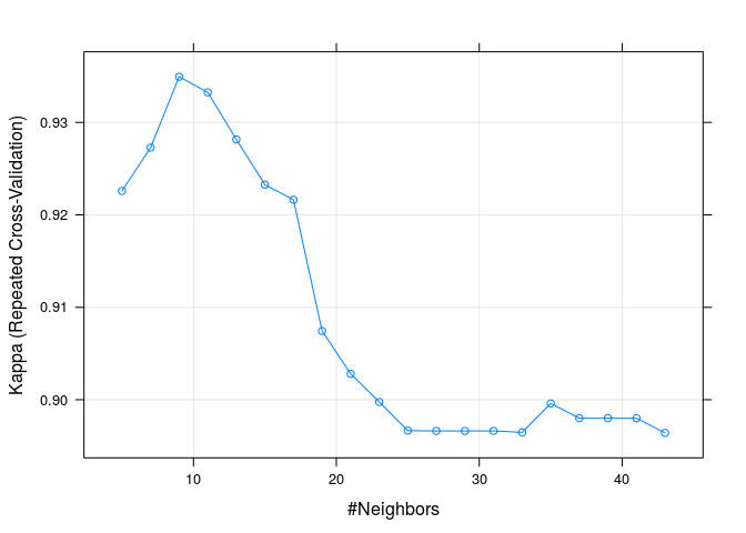
Kappa was used to select the optimal model using the largest value.
The final value used for the model was k = 9.
plot(knnFit2)
knnPredict2 <- predict(knnFit2, newdata=wdbc_test)
cmat2 <- confusionMatrix(knnPredict2, wdbc_test$diagnosis, positive="Malignant")
cmat2
Confusion Matrix and Statistics

           Reference
Prediction  Benign Malignant
  Benign        61         4
  Malignant      0        35

               Accuracy : 0.96
                 95% CI : (0.901, 0.989)
    No Information Rate : 0.61
    P-Value [Acc > NIR] : 2.39e-16

                  Kappa : 0.914
 Mcnemar's Test P-Value : 0.134

            Sensitivity : 0.897
            Specificity : 1.000
         Pos Pred Value : 1.000
         Neg Pred Value : 0.938
             Prevalence : 0.390
         Detection Rate : 0.350
   Detection Prevalence : 0.350
      Balanced Accuracy : 0.949

       'Positive' Class : Malignant
Now, instead of a k=13 of the first model, we
have a k=9 when using kappa.
Using ROC as metric
Finally, let’s consider using the ROC metric, for that we need to change
the control parameters:
ctrl <- trainControl(method="repeatedcv", number=10, repeats=3,
                     classProbs=TRUE, summaryFunction=twoClassSummary)
knnFit3 <- train(diagnosis ~ ., data=wdbc_train, method="knn",
                trControl=ctrl, metric="ROC", tuneLength=30,
                preProc=c("range"))
knnFit3
k-Nearest Neighbors
469 samples
30 predictors
2 classes: 'Benign', 'Malignant'
Pre-processing: re-scaling to [0, 1]
Resampling: Cross-Validated (10 fold, repeated 3 times)
Summary of sample sizes: 421, 421, 423, 423, 422, 422, ...
Resampling results across tuning parameters:
k ROC Sens Spec ROC SD Sens SD Spec SD
5 0.9854 0.9818 0.9268 0.02040 0.02805 0.06620
7 0.9877 0.9841 0.9327 0.01920 0.02655 0.06306
9 0.9898 0.9875 0.9310 0.01513 0.02279 0.06295
11 0.9907 0.9898 0.9310 0.01342 0.01819 0.06938
13 0.9897 0.9932 0.9309 0.01430 0.01634 0.06992
15 0.9900 0.9933 0.9214 0.01383 0.02039 0.06980
17 0.9896 0.9921 0.9059 0.01411 0.02284 0.06996
19 0.9892 0.9899 0.9039 0.01412 0.02180 0.07612
21 0.9888 0.9899 0.8963 0.01466 0.02180 0.08064
23 0.9890 0.9899 0.8943 0.01464 0.02180 0.08022
25 0.9889 0.9854 0.8904 0.01478 0.02447 0.08073
27 0.9888 0.9888 0.8904 0.01481 0.02393 0.07616
29 0.9884 0.9910 0.8904 0.01518 0.02142 0.07616
31 0.9885 0.9910 0.8924 0.01511 0.02142 0.07353
33 0.9886 0.9899 0.8942 0.01475 0.02180 0.07555
35 0.9889 0.9910 0.8904 0.01454 0.02142 0.07616
37 0.9888 0.9889 0.8904 0.01474 0.02207 0.07616
39 0.9889 0.9900 0.8904 0.01489 0.02175 0.07616
41 0.9886 0.9922 0.8885 0.01486 0.02092 0.07866
43 0.9886 0.9911 0.8885 0.01483 0.02137 0.07866
45 0.9883 0.9900 0.8885 0.01516 0.02175 0.07866
47 0.9881 0.9866 0.8845 0.01511 0.02256 0.08329
49 0.9878 0.9888 0.8865 0.01547 0.02211 0.08103
51 0.9877 0.9899 0.8827 0.01540 0.02180 0.08506
53 0.9878 0.9922 0.8808 0.01523 0.01680 0.07991
55 0.9877 0.9922 0.8846 0.01544 0.01680 0.08145
57 0.9875 0.9922 0.8790 0.01558 0.01680 0.08183
59 0.9873 0.9900 0.8789 0.01569 0.01789 0.08492
61 0.9874 0.9900 0.8771 0.01580 0.01789 0.08770
63 0.9872 0.9911 0.8790 0.01589 0.01736 0.08854
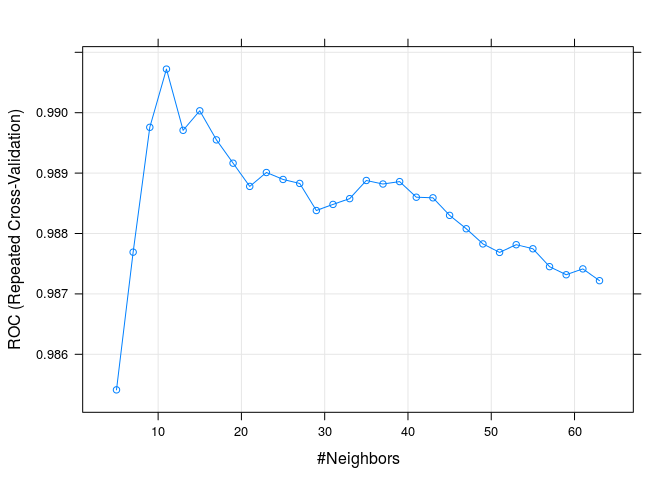
ROC was used to select the optimal model using the largest value.
The final value used for the model was k = 11.
plot(knnFit3)
knnPredict3 <- predict(knnFit3, newdata=wdbc_test)
cmat3 <- confusionMatrix(knnPredict3, wdbc_test$diagnosis, positive="Malignant")
cmat3
Confusion Matrix and Statistics

           Reference
Prediction  Benign Malignant
  Benign        61         3
  Malignant      0        36

               Accuracy : 0.97
                 95% CI : (0.915, 0.994)
    No Information Rate : 0.61
    P-Value [Acc > NIR] : <2e-16

                  Kappa : 0.936
 Mcnemar's Test P-Value : 0.248

            Sensitivity : 0.923
            Specificity : 1.000
         Pos Pred Value : 1.000
         Neg Pred Value : 0.953
             Prevalence : 0.390
         Detection Rate : 0.360
   Detection Prevalence : 0.360
      Balanced Accuracy : 0.962

       'Positive' Class : Malignant
For the ROC metric the best model is for k=11.
Comparing the three models
Just to have a clear understanding of the differences between the three kNN models, we will summarize them in a table. We’ll also include the data from the book’s example.
# from the book's table in page 83
tn=61
tp=37
fn=2
fp=0
book_example <- list(
    k=21,
    metric=NA,
    value=NA,
    TN=tn,
    TP=tp,
    FN=fn,
    FP=fp,
    acc=(tp + tn)/(tp + tn + fp + fn),
    sens=tp/(tp + fn),
    spec=tn/(tn + fp),
    PPV=tp/(tp + fp),
    NPV=tn/(tn + fn))

model_comp <- as.data.frame(
    rbind(round_numeric(book_example),
          summod(cmat1, knnFit1),
          summod(cmat2, knnFit2),
          summod(cmat3, knnFit3)))
rownames(model_comp) <- c("Book model", "Model 1", "Model 2", "Model 3")
pander(model_comp[,-3], split.tables=Inf, keep.trailing.zeros=TRUE,
       style="rmarkdown",
       caption="Model results when comparing predictions and test set")
Model results when comparing predictions and test set
| k | metric | TN | TP | FN | FP | acc | sens | spec | PPV | NPV | |
|---|---|---|---|---|---|---|---|---|---|---|---|
| Book model | 21 | 61 | 37 | 2 | 0 | 0.98 | 0.95 | 1 | 1 | 0.97 | |
| Model 1 | 13 | Accuracy | 61 | 36 | 3 | 0 | 0.97 | 0.92 | 1 | 1 | 0.95 |
| Model 2 | 9 | Kappa | 61 | 35 | 4 | 0 | 0.96 | 0.9 | 1 | 1 | 0.94 |
| Model 3 | 11 | ROC | 61 | 36 | 3 | 0 | 0.97 | 0.92 | 1 | 1 | 0.95 |
The book’s model using 21 neighbours is a tad better in accuracy, sensitivity
and NPV. So it tends to make fewer Type II errors than the other models. On the
other hand, it uses almost twice as many neighbours as any of the models
estimated using caret.
Overall it seems that, with caret and in this particular case, it is almost the
same whether we use Accuracy or ROC as the selection metric, as both give
similar results.
Changing the data partition strategy
A question remains as to whether a different partition strategy will improve or
not the caret models. So we will try three different data partition strategies
using the Accuracy metric.
We will choose the following data partitions (ratio of training:testing cases):
- Model A: 469:100 (the proportion used in the book)
- Model B: 1:1 (50% training, 50% testing)
- Model C: 9:1 (90% training, 10% testing)
Using the book’s proportions
We will use the proportion of 469:100 to partition the data (~82.425% of rows for training) trying to keep the proportions of diagnosis similar in the in all sets. To show that this latter condition is kept, we will compare the proportions of diagnosis in the original, training and testing data sets.
set.seed(12345)
ptr <- 469/569
train_index <- createDataPartition(wdbc$diagnosis, p=ptr, list=FALSE)
wdbc_train <- wdbc[train_index,]
wdbc_test <- wdbc[-train_index,]
ft_train <- frqtab(wdbc_train$diagnosis)
ft_test <- frqtab(wdbc_test$diagnosis)
ft_df <- as.data.frame(cbind(ft_orig, ft_train, ft_test))
colnames(ft_df) <- c("Original", "Training set", "Test set")
pander(ft_df, style="rmarkdown",
       caption=paste0("Comparison of diagnosis frequencies for prop(train)=",
                      round(ptr*100, 2),"%"))
Comparison of diagnosis frequencies for prop(train)=82.43%
| Original | Training set | Test set | |
|---|---|---|---|
| Benign | 62.7 | 62.8 | 62.6 |
| Malignant | 37.3 | 37.2 | 37.4 |
Now let’s calculate the model using Accuracy as selection metric:
ctrl <- trainControl(method="repeatedcv", number=10, repeats=3)
set.seed(12345)
knnFitA <- train(diagnosis ~ ., data=wdbc_train, method="knn",
trControl=ctrl, metric="Accuracy", tuneLength=20,
preProc=c("range"))
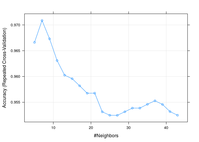
plot(knnFitA)
knnPredictA <- predict(knnFitA, newdata=wdbc_test)
cmatA <- confusionMatrix(knnPredictA, wdbc_test$diagnosis, positive="Malignant")
cmatA
Confusion Matrix and Statistics

           Reference
Prediction  Benign Malignant
  Benign        62         4
  Malignant      0        33

               Accuracy : 0.96
                 95% CI : (0.9, 0.989)
    No Information Rate : 0.626
    P-Value [Acc > NIR] : 3.88e-15

                  Kappa : 0.912
 Mcnemar's Test P-Value : 0.134

            Sensitivity : 0.892
            Specificity : 1.000
         Pos Pred Value : 1.000
         Neg Pred Value : 0.939
             Prevalence : 0.374
         Detection Rate : 0.333
   Detection Prevalence : 0.333
      Balanced Accuracy : 0.946

       'Positive' Class : Malignant
This time we have a different number or neigbours (k=7), but our accuracy is not as good (0.96) and also the sensitivity has decreased (0.89) because we have more false negatives.
Using the 1:1 training:testing proportion
set.seed(12345)
ptr <- .5
train_index <- createDataPartition(wdbc$diagnosis, p=ptr, list=FALSE)
wdbc_train <- wdbc[train_index,]
wdbc_test <- wdbc[-train_index,]
set.seed(12345)
knnFitB <- train(diagnosis ~ ., data=wdbc_train, method="knn",
                trControl=ctrl, metric="Accuracy", tuneLength=20,
                preProc=c("range"))
knnPredictB <- predict(knnFitB, newdata=wdbc_test)
cmatB <- confusionMatrix(knnPredictB, wdbc_test$diagnosis, positive="Malignant")
cmatB
Confusion Matrix and Statistics

           Reference
Prediction  Benign Malignant
  Benign       174         4
  Malignant      4       102

               Accuracy : 0.972
                 95% CI : (0.945, 0.988)
    No Information Rate : 0.627
    P-Value [Acc > NIR] : <2e-16

                  Kappa : 0.94
 Mcnemar's Test P-Value : 1

            Sensitivity : 0.962
            Specificity : 0.978
         Pos Pred Value : 0.962
         Neg Pred Value : 0.978
             Prevalence : 0.373
         Detection Rate : 0.359
   Detection Prevalence : 0.373
      Balanced Accuracy : 0.970

       'Positive' Class : Malignant
Using 50% of the cases for training, gives us a model using k=9 nearest neighbours, with an accuracy of 0.97 and a sensitivity of 0.96
Using the 9:1 training:testing proportion
set.seed(12345)
ptr <- .9
train_index <- createDataPartition(wdbc$diagnosis, p=ptr, list=FALSE)
wdbc_train <- wdbc[train_index,]
wdbc_test <- wdbc[-train_index,]
set.seed(12345)
knnFitC <- train(diagnosis ~ ., data=wdbc_train, method="knn",
                trControl=ctrl, metric="Accuracy", tuneLength=20,
                preProc=c("range"))
knnPredictC <- predict(knnFitC, newdata=wdbc_test)
cmatC <- confusionMatrix(knnPredictC, wdbc_test$diagnosis, positive="Malignant")
cmatC
Confusion Matrix and Statistics

           Reference
Prediction  Benign Malignant
  Benign        35         3
  Malignant      0        18

               Accuracy : 0.946
                 95% CI : (0.851, 0.989)
    No Information Rate : 0.625
    P-Value [Acc > NIR] : 2.44e-08

                  Kappa : 0.882
 Mcnemar's Test P-Value : 0.248

            Sensitivity : 0.857
            Specificity : 1.000
         Pos Pred Value : 1.000
         Neg Pred Value : 0.921
             Prevalence : 0.375
         Detection Rate : 0.321
   Detection Prevalence : 0.321
      Balanced Accuracy : 0.929

       'Positive' Class : Malignant
Using 90% of the cases for training, gives us a model using k=5 nearest neighbours, with an accuracy of 0.95 and a sensitivity of 0.86
Comparing the models from different partition strategies
As we have used the same random seed for all models, we can compare them in equal footing.
We will compare:
- Model 1
- Data was partitioned using the first 469 rows for training, and the other 100 rows for testing
- Model A
- Data was partitioned using the same 469:100 proportion, but trying to maintain a distribution of diagnosis similar to the full data set in the training and testing sets
- Model B
- Data was partitioned 50% for training and 50% for testing, and trying to maintain the same distribution of diagnosis in the training and testing set as the original data.
- Model C
- Data was partitioned 90% for training and 10% for testing, while trying to maintain the same distribution of diagnosis in the training and testing set as the original data.
model_comp <- data.frame(
    rbind(
        summod(cmat1, knnFit1),
        summod(cmatA, knnFitA),
        summod(cmatB, knnFitB),
        summod(cmatC, knnFitC)
        )
    )
rownames(model_comp) <- c("Model 1", "Model A", "Model B", "Model C")
pander(model_comp[,-c(2,3)], split.tables=Inf, keep.trailing.zeros=TRUE,
       style="rmarkdown",
       caption="Model comparison using different data partitioning proportions")
Model comparison using different data partitioning proportions
| k | TN | TP | FN | FP | acc | sens | spec | PPV | NPV | |
|---|---|---|---|---|---|---|---|---|---|---|
| Model 1 | 13 | 61 | 36 | 3 | 0 | 0.97 | 0.92 | 1 | 1 | 0.95 |
| Model A | 7 | 62 | 33 | 4 | 0 | 0.96 | 0.89 | 1 | 1 | 0.94 |
| Model B | 9 | 174 | 102 | 4 | 4 | 0.97 | 0.96 | 0.98 | 0.96 | 0.98 |
| Model C | 5 | 35 | 18 | 3 | 0 | 0.95 | 0.86 | 1 | 1 | 0.92 |
Comparing Model 1 and Model A, we find that using a balanced proportion of diagnosis in the testing and training sets, has the effect of reducing the number of nearest neighbours to almost half (from 13 to 7), but also impacts slightly the accuracy, and the related measures of sensitivity and NPV.
Using a 1:1 training:testing proportion (Model B), affords a slightly better accuracy and sensitivity, but at the expense of decreasing the specificity. This might be a good trade-off in this case, having fewer false negatives will save more lives, which more than compensates the occurence of a few more false positives.
Finally, using 90% for training and 10% for testing not only reduces the number of nearest neigbors needed in the model, but also increases the proportion of false negatives, decreasing its sensitivity and NPV.
Reproducibility information
The dataset used is the modified version of the “Breast Cancer Wisconsin (Diagnostic) Data Set” from the UCI Machine Learning Repository, as described in the book “Machine Learning with R” by Brett Lantz (ISBN 978-1-78216-214-8).
sessionInfo()
R version 3.1.2 (2014-10-31)
Platform: x86_64-pc-linux-gnu (64-bit)

locale:
 [1] LC_CTYPE=en_US.UTF-8       LC_NUMERIC=C
 [3] LC_TIME=en_US.UTF-8        LC_COLLATE=en_US.UTF-8
 [5] LC_MONETARY=en_US.UTF-8    LC_MESSAGES=en_US.UTF-8
 [7] LC_PAPER=en_US.UTF-8       LC_NAME=C
 [9] LC_ADDRESS=C               LC_TELEPHONE=C
[11] LC_MEASUREMENT=en_US.UTF-8 LC_IDENTIFICATION=C

attached base packages:
[1] parallel  stats     graphics  grDevices utils     datasets  methods
[8] base

other attached packages:
[1] pROC_1.7.3      pander_0.3.8    doMC_1.3.3      iterators_1.0.7
[5] foreach_1.4.2   caret_6.0-37    ggplot2_1.0.0   lattice_0.20-29
[9] knitr_1.6

loaded via a namespace (and not attached):
 [1] BradleyTerry2_1.0-5 brglm_0.5-9         car_2.0-19
 [4] class_7.3-11        codetools_0.2-9     colorspace_1.2-2
 [7] compiler_3.1.2      digest_0.6.4        e1071_1.6-4
[10] evaluate_0.5.5      formatR_0.10        grid_3.1.2
[13] gtable_0.1.2        gtools_3.4.1        htmltools_0.2.6
[16] lme4_1.1-6          MASS_7.3-35         Matrix_1.1-4
[19] minqa_1.2.3         munsell_0.4.2       nlme_3.1-118
[22] nnet_7.3-8          plyr_1.8.1          proto_0.3-10
[25] Rcpp_0.11.3         RcppEigen_0.3.2.1.2 reshape2_1.4
[28] rmarkdown_0.3.3     scales_0.2.4        splines_3.1.2
[31] stringr_0.6.2       tools_3.1.2         yaml_2.1.11
Notes:
- This was also published at RPubs: http://rpubs.com/jesuscastagnetto/caret-knn-cancer-prediction
- You can get the source code for the .Rmd file at: https://github.com/jmcastagnetto/examples-from-mlwr/tree/master/ch03
- Book page at Packt [return]
- The caret package site [return]
- http://cran.r-project.org/web/packages/class/index.html [return]
- https://archive.ics.uci.edu/ml/datasets/Breast+Cancer+Wisconsin+%28Diagnostic%29 [return]
- Implemented in the function
knn3incaret. [return]