Compare simulated mean and variance with the theoretical values
We will run 1000 rounds of simulation of 40 exponentials with \( \lambda = 0.2 \), using a fixed seed, and comparing the center of the distribution of the mean and variance values with the theoretical \( 1 / \lambda \).
 1 library(ggplot2)
 2 library(knitr)
 3
 4 nsim <- 1000
 5 nvals <- 40
 6 lambda <- 0.2
 7 set.seed(567)
 8 simdata <- t(replicate(nsim, rexp(nvals, lambda)))
 9 df <- data.frame(Mean=c(mean(rowMeans(simdata)), 1/lambda),
10                  Variance=c(mean(apply(simdata, 1, var)), 1/lambda^2))
11 rownames(df) <- c("Simulated", "Theoretical")
12 kable(df)
| Mean | Variance | |
|---|---|---|
| Simulated | 4.99 | 24.78 |
| Theoretical | 5.00 | 25.00 |
The simulated and theoretical values are very close, as expected by the CLT.
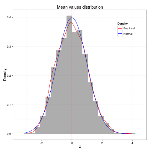
Assess if the simulated values are approximately normal
Also, according to the CLT, the distribution of the simulated means should be approximately normal. To illustrate this we will normalize the vectors and compare it to a \( N(0,1) \) distribution.
 1 meanvals <- rowMeans(simdata)
 2 zmean <- (meanvals - mean(meanvals)) / sd(meanvals)
 3 qplot(zmean, geom = "blank") +
 4     geom_line(aes(y = ..density.., colour = 'Empirical'), stat = 'density') +
 5     stat_function(fun = dnorm, aes(colour = 'Normal')) +
 6     geom_histogram(aes(y = ..density..), alpha = 0.4, binwidth=.35) +
 7     geom_vline(xintercept=0, colour="red", linetype="longdash") +
 8     scale_colour_manual(name = 'Density', values = c('red', 'blue')) +
 9     ylab("Density") + xlab("z") + ggtitle("Mean values distribution") +
10     theme_bw() + theme(legend.position = c(0.85, 0.85))
Evaluate the coverage of the confidence interval
Theoretically, a 95% confidence interval should contain, if we simulate a big number of them, the mean value for the exponential distribution \( 1 / \lambda \) ) 95% of the time.
 1 set.seed(567)
 2 lambda <- 0.2
 3 # checks for each simulation if the mean is in the confidence interval
 4 inconfint <- function(lambda) {
 5                 ehats <- rexp(1000, lambda)
 6                 se <- sd(ehats)/sqrt(1000)
 7                 ll <- mean(ehats) - 1.96 * se
 8                 ul <- mean(ehats) + 1.96 * se
 9                 (ll < 1/lambda & ul > 1/lambda)
10         }
11 # estimate the coverage in each round of simulations
12 coverage <- function(lambda) {
13     covvals <- replicate(100, inconfint(lambda))
14     mean(covvals)
15 }
16 # perform the simulation
17 simres <- replicate(100, coverage(lambda))
18 mean(simres)
## [1] 0.9484
As expected, the confidence interval contains the theoretical value 94.84% of the time (close to the expected 95%).